Clustering

Clustering techniques are unsupervised algorithms that try to group unlabelled data into “clusters”, using the (typically spatial) structure of the data itself. It has many applications.

The easiest way to demonstrate how clustering works is to simply generate some data and show them in action. We’ll start off by importing the libraries we’ll be using today.

import math, matplotlib.pyplot as plt, operator, torch
from functools import partial
/Users/anubhavmaity/mambaforge/envs/fastai/lib/python3.9/site-packages/tqdm/auto.py:22: TqdmWarning: IProgress not found. Please update jupyter and ipywidgets. See https://ipywidgets.readthedocs.io/en/stable/user_install.html
  from .autonotebook import tqdm as notebook_tqdm
torch.manual_seed(42)
torch.set_printoptions(precision=3, linewidth=140, sci_mode=False)

Create data

n_clusters = 6
n_samples = 250

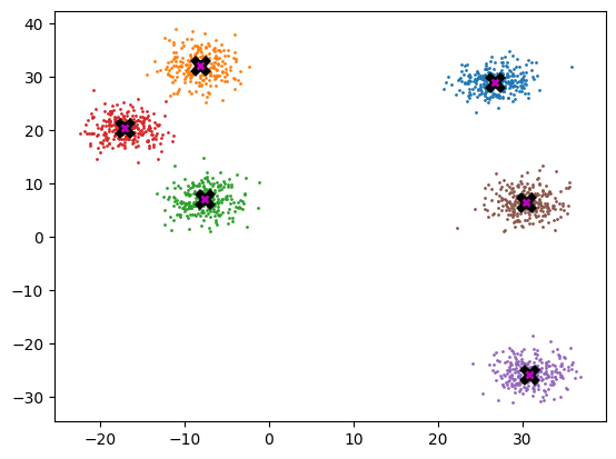
To generate our data, we are going back to pick 6 random points, which we will call centroids, and for each point we are going to generate 250 random points about it.

centroids = torch.rand(n_clusters, 2) * 70 - 35
centroids
tensor([[ 26.759,  29.050],
        [ -8.200,  32.151],
        [ -7.669,   7.063],
        [-17.040,  20.555],
        [ 30.854, -25.677],
        [ 30.422,   6.551]])
from torch.distributions.multivariate_normal import MultivariateNormal
from torch import tensor
def sample(m): return MultivariateNormal(m, torch.diag(tensor([5., 5.]))).sample((n_samples, ))
slices = [sample(c) for c in centroids]
data  = torch.cat(slices)
data.shape
torch.Size([1500, 2])

Below we can see each centroid marked w/X, and the coloring associated to each respective cluster.

def plot_data(centroids, data, n_samples, ax=None):
    if ax is None: _, ax = plt.subplots()
    for i, centroid in enumerate(centroids):
        samples = data[i*n_samples: (i+1)*n_samples]
        ax.scatter(samples[:, 0], samples[:, 1], s=1)
        ax.plot(*centroid, markersize=10, marker="x", color='k', mew=5)
        ax.plot(*centroid, markersize=5, marker="x", color='m', mew=2)
plot_data(centroids, data, n_samples)

Mean Shift

Most people that have come across clustering algorithms have learnt about k-means. Mean shift clustering is a newer and less well-known approach, but it has some important advantages: - It doesn’t require selecting the number of clusters in advance, but instead just requires a bandwidth to be specified, which can be easily chosen automatically. - It can handle clusters of any shape, whereas k-means (without using special extensions) requires that clusters be roughly ball shaped

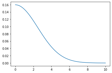
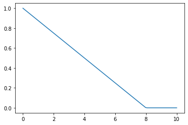
The algorithm is as follows: - For each data point x in the sample X, find the distance between that point x and every other point in X - Create weights for each point in X by using the Gaussian kernel of that point’s distance to x - This weighting approach penalizes points further away from x - The rate at which the weights fall to zero is determined by the bandwidth, which is the standard deviation of the Gaussian - Update x as the weighted all other points in X, weighted based on the previous step

This will iteratively push points that are close together even closer until they are next to each other
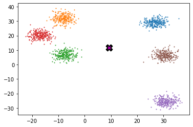
midp = data.mean(0)
midp
tensor([ 9.222, 11.604])
plot_data([midp]*6, data, n_samples)

So here is the definition of the gaussian kernel, which you may remember from high school..

\[ \frac{1}{\sqrt{ 2 \pi \sigma^2 }} \exp\biggl( - \frac{ (x - \mu)^2 } {2 \sigma^2} \biggr) \]

def gaussian(d, bw): return torch.exp(-0.5*((d/bw))**2) / (bw*math.sqrt(2*math.pi))
def plot_func(f):
    x = torch.linspace(0, 10, 100)
    plt.plot(x, f(x))
plot_func(partial(gaussian, bw=2.5))

partial
functools.partial

In our implementation, we choose the bandwidth to be 2.5

One easy way to choose bandwidth is to find which bandwidth covers one thid of the data

def tri(d, i): return (-d + i).clamp_min(0)/i
plot_func(partial(tri, i=8))

X = data.clone()
x = data[0]
x
tensor([26.204, 26.349])
x.shape, X.shape, x[None].shape
(torch.Size([2]), torch.Size([1500, 2]), torch.Size([1, 2]))
(x[None] - X)[:8]
tensor([[ 0.000,  0.000],
        [ 0.513, -3.865],
        [-4.227, -2.345],
        [ 0.557, -3.685],
        [-5.033, -3.745],
        [-4.073, -0.638],
        [-3.415, -5.601],
        [-1.920, -5.686]])
(x - X)[:8]
tensor([[ 0.000,  0.000],
        [ 0.513, -3.865],
        [-4.227, -2.345],
        [ 0.557, -3.685],
        [-5.033, -3.745],
        [-4.073, -0.638],
        [-3.415, -5.601],
        [-1.920, -5.686]])
dist = ((x-X)**2).sum(1).sqrt()
dist[:8]
tensor([0.000, 3.899, 4.834, 3.726, 6.273, 4.122, 6.560, 6.002])
((x-X)**2).sum(1)
tensor([  0.000,  15.199,  23.369,  ..., 310.729, 511.192, 467.316])

rewrite using torch.einsum

torch.einsum('ik,ik->i',x-X, x-X).sqrt()
tensor([ 0.000,  3.899,  4.834,  ..., 17.628, 22.610, 21.617])
weight = gaussian(dist, 2.5)
weight
tensor([    0.160,     0.047,     0.025,  ...,     0.000,     0.000,     0.000])
weight.shape, X.shape
(torch.Size([1500]), torch.Size([1500, 2]))
weight[:, None].shape
torch.Size([1500, 1])
weight[:, None] * X
tensor([[    4.182,     4.205],
        [    1.215,     1.429],
        [    0.749,     0.706],
        ...,
        [    0.000,     0.000],
        [    0.000,     0.000],
        [    0.000,     0.000]])
def one_update(X):
    for i, x in enumerate(X):
        dist = torch.sqrt(((x - X)**2).sum(1))
#         weight = gaussian(dist, 2.5)
        weight = tri(dist, 8)
        X[i] = (weight[:, None] * X).sum(0)/weight.sum()
def meanshift(data):
    X = data.clone()
    for it in range(5): one_update(X)
    return X
CPU times: user 470 ms, sys: 0 ns, total: 470 ms
Wall time: 470 ms
plot_data(centroids + 2, X, n_samples)

Animation

from matplotlib.animation import FuncAnimation
from IPython.display import HTML
def do_one(d):
    if not d: return plot_data(centroids + 2, X, n_samples, ax=ax)
    one_update(X)
    ax.clear()
    plot_data(centroids + 2, X, n_samples, ax=ax)
X = data.clone()
fig,ax = plt.subplots()
ani = FuncAnimation(fig, do_one, frames=5, interval=500, repeat=False)
plt.close()
HTML(ani.to_jshtml())

animation for your own algorithm

GPU batched algorithm

To truly accelerate the algorithm, we need to be performing updates on a batch of points per iteration, instead of just one as were doing

bs = 5
X = data.clone()
x = X[:bs]
x.shape, X.shape
(torch.Size([5, 2]), torch.Size([1500, 2]))
def dist_b(a, b): return torch.sqrt(((a[None] - b[:, None])**2).sum(2))
dist_b(X, x)
tensor([[ 0.000,  3.899,  4.834,  ..., 17.628, 22.610, 21.617],
        [ 3.899,  0.000,  4.978,  ..., 21.499, 26.508, 25.500],
        [ 4.834,  4.978,  0.000,  ..., 19.373, 24.757, 23.396],
        [ 3.726,  0.185,  4.969,  ..., 21.335, 26.336, 25.333],
        [ 6.273,  5.547,  1.615,  ..., 20.775, 26.201, 24.785]])
dist_b(X, x).shape
torch.Size([5, 1500])
X[None, :].shape, x[:, None].shape, (X[None, :] - x[:, None]).shape
(torch.Size([1, 1500, 2]), torch.Size([5, 1, 2]), torch.Size([5, 1500, 2]))
weight = gaussian(dist_b(X, x), 2)
weight
tensor([[    0.199,     0.030,     0.011,  ...,     0.000,     0.000,     0.000],
        [    0.030,     0.199,     0.009,  ...,     0.000,     0.000,     0.000],
        [    0.011,     0.009,     0.199,  ...,     0.000,     0.000,     0.000],
        [    0.035,     0.199,     0.009,  ...,     0.000,     0.000,     0.000],
        [    0.001,     0.004,     0.144,  ...,     0.000,     0.000,     0.000]])
weight.shape, X.shape
(torch.Size([5, 1500]), torch.Size([1500, 2]))
weight[..., None].shape, X[None].shape
(torch.Size([5, 1500, 1]), torch.Size([1, 1500, 2]))
num = (weight[..., None]*X[None]).sum(1)
num.shape
torch.Size([5, 2])
num
tensor([[367.870, 386.231],
        [518.332, 588.680],
        [329.665, 330.782],
        [527.617, 598.217],
        [231.302, 234.155]])
torch.einsum('ij,jk->ik', weight, X)
tensor([[367.870, 386.231],
        [518.332, 588.680],
        [329.665, 330.782],
        [527.617, 598.217],
        [231.302, 234.155]])
weight@X
tensor([[367.870, 386.231],
        [518.332, 588.680],
        [329.665, 330.782],
        [527.617, 598.217],
        [231.302, 234.155]])
div = weight.sum(1, keepdim=True)
div.shape
torch.Size([5, 1])
num/div
tensor([[26.376, 27.692],
        [26.101, 29.643],
        [28.892, 28.990],
        [26.071, 29.559],
        [29.323, 29.685]])
def meanshift(data, bs=500):
    n = len(data)
    X = data.clone()
    for it in range(5):
        for i in range(0, n, bs):
            s = slice(i, min(i+bs, n))
            weight = gaussian(dist_b(X, X[s]), 2.5)
            div = weight.sum(1, keepdim=True)
            X[s] = weight@X/div
    return X

Although each iteration still has to launch a new cuda kernel, there are now fewer iterations, and the acceleration from updating a batch of points more than makes up for it.

data = data.cuda()
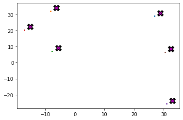
X = meanshift(data).cpu()
2.25 ms ± 36 µs per loop (mean ± std. dev. of 7 runs, 5 loops each)
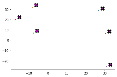
plot_data(centroids + 2, X, n_samples)

45 ms ± 654 µs per loop (mean ± std. dev. of 7 runs, 5 loops each)