from collections import Counter
import numpy as np
import torch
from rich import print
from rich import pretty
from matplotlib import pyplot as pltBuilding makemore
The spelled-out intro to language modeling
g = torch.Generator().manual_seed(2147483647)pretty.install()Counting
Read in the data
def get_words(filename):
    with open('../data/names.txt') as f:
        return list(map(lambda x: x.strip(), f.readlines()))
words = get_words('../data/names.txt')words[:10]['emma', 'olivia', 'ava', 'isabella', 'sophia', 'charlotte', 'mia', 'amelia', 'harper', 'evelyn']
len(words)32033
Minimum Length
min(len(w) for w in words)2
Maximum Length
max(len(w) for w in words)15
Create paring of nth and n + 1th position characters
for w in words[:1]:
    for ch1, ch2 in zip(w, w[1:]):
        print(ch1, ch2)
e m
m m
m a
Add start (<S>) and end(<E>) tokens to the word
The model will know the starting and ending of the word
def generate_pairings(words, start_token='<S>', end_token='<E>'):
    for w in words:
        chs = [start_token] + list(w) + [end_token]
        for ch1, ch2 in zip(chs, chs[1:]):
            yield ch1, ch2
for ch1, ch2 in generate_pairings(words[:1]):
print(ch1, ch2)<S> e
e m
m m
m a
a <E>
sum(1 for ch1, ch2 in generate_pairings(words))228146
lets see for 3 words
for ch1, ch2 in generate_pairings(words[:3]):
print(ch1, ch2)<S> e
e m
m m
m a
a <E>
<S> o
o l
l i
i v
v i
i a
a <E>
<S> a
a v
v a
a <E>
Count of bigrams
Bigram for 3 words
def create_bigram_counter(words):
    b = Counter()
    for ch1, ch2 in generate_pairings(words):
        bigram = (ch1, ch2)
        b[bigram] += 1
return bcreate_bigram_counter(words[:3])Counter({ ('<S>', 'e'): 1, ('e', 'm'): 1, ('m', 'm'): 1, ('m', 'a'): 1, ('a', '<E>'): 3, ('<S>', 'o'): 1, ('o', 'l'): 1, ('l', 'i'): 1, ('i', 'v'): 1, ('v', 'i'): 1, ('i', 'a'): 1, ('<S>', 'a'): 1, ('a', 'v'): 1, ('v', 'a'): 1 })
Bigram for all words
b = create_bigram_counter(words)b.most_common(10)[ (('n', '<E>'), 6763), (('a', '<E>'), 6640), (('a', 'n'), 5438), (('<S>', 'a'), 4410), (('e', '<E>'), 3983), (('a', 'r'), 3264), (('e', 'l'), 3248), (('r', 'i'), 3033), (('n', 'a'), 2977), (('<S>', 'k'), 2963) ]
Create 2D array of the bigram
Little warmup with tensors
a = torch.zeros((3, 5), dtype=torch.int32)
atensor([[0, 0, 0, 0, 0], [0, 0, 0, 0, 0], [0, 0, 0, 0, 0]], dtype=torch.int32)
a.dtypetorch.int32
a[1,3] = 1
atensor([[0, 0, 0, 0, 0], [0, 0, 0, 1, 0], [0, 0, 0, 0, 0]], dtype=torch.int32)
a[1, 3] += 1
atensor([[0, 0, 0, 0, 0], [0, 0, 0, 2, 0], [0, 0, 0, 0, 0]], dtype=torch.int32)
2D matrix of alpahabets
def get_stoi(words, start_token, end_token, tokens_at_start=True):
    chars = []
    if tokens_at_start:
        chars.append(start_token)
        if start_token != end_token: chars.append(end_token)

    chars.extend(sorted(list(set(''.join(words)))))

    if not tokens_at_start:
        chars.append(start_token)
        if start_token != end_token: chars.append(end_token)

    stoi = {s:i for i,s in enumerate(chars)}

    return stoi
stoi = get_stoi(words, '<S>', '<E>', tokens_at_start=False)
stoi{ 'a': 0, 'b': 1, 'c': 2, 'd': 3, 'e': 4, 'f': 5, 'g': 6, 'h': 7, 'i': 8, 'j': 9, 'k': 10, 'l': 11, 'm': 12, 'n': 13, 'o': 14, 'p': 15, 'q': 16, 'r': 17, 's': 18, 't': 19, 'u': 20, 'v': 21, 'w': 22, 'x': 23, 'y': 24, 'z': 25, '<S>': 26, '<E>': 27 }
def create_bigram_matrix(words, start_token, end_token, tokens_at_start=True):
    stoi = get_stoi(words, start_token, end_token, tokens_at_start)
    alphabet_size = len(stoi)
    N = torch.zeros((alphabet_size, alphabet_size), dtype=torch.int32)
    for ch1, ch2 in generate_pairings(words, start_token, end_token):
        ix1 = stoi[ch1]
        ix2 = stoi[ch2]
        N[ix1, ix2] += 1
    return N
N = create_bigram_matrix(words, '<S>', '<E>', False)N[:10, :10]tensor([[ 556, 541, 470, 1042, 692, 134, 168, 2332, 1650, 175], [ 321, 38, 1, 65, 655, 0, 0, 41, 217, 1], [ 815, 0, 42, 1, 551, 0, 2, 664, 271, 3], [1303, 1, 3, 149, 1283, 5, 25, 118, 674, 9], [ 679, 121, 153, 384, 1271, 82, 125, 152, 818, 55], [ 242, 0, 0, 0, 123, 44, 1, 1, 160, 0], [ 330, 3, 0, 19, 334, 1, 25, 360, 190, 3], [2244, 8, 2, 24, 674, 2, 2, 1, 729, 9], [2445, 110, 509, 440, 1653, 101, 428, 95, 82, 76], [1473, 1, 4, 4, 440, 0, 0, 45, 119, 2]], dtype=torch.int32)
The type of a cell in the above N is tensor
type(N[1, 1])<class 'torch.Tensor'>
Therefore we have to call it with .item() to get the value
type(N[1, 1].item())<class 'int'>
plt.imshow(N)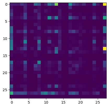
itos = dict(map(reversed, stoi.items()))
itos
{ 0: 'a', 1: 'b', 2: 'c', 3: 'd', 4: 'e', 5: 'f', 6: 'g', 7: 'h', 8: 'i', 9: 'j', 10: 'k', 11: 'l', 12: 'm', 13: 'n', 14: 'o', 15: 'p', 16: 'q', 17: 'r', 18: 's', 19: 't', 20: 'u', 21: 'v', 22: 'w', 23: 'x', 24: 'y', 25: 'z', 26: '<S>', 27: '<E>' }
def plot_matrix(N, itos):
    plt.figure(figsize=(16, 16))
    plt.imshow(N, cmap='Blues')
    for i in range(N.shape[0]):
        for j in range(N.shape[1]):
            chstr = itos[i] + itos[j]
            plt.text(j, i, chstr, ha="center", va="bottom", color="gray")
            plt.text(j, i, N[i, j].item(), ha="center", va="top", color="gray")
    plt.axis("off")
plot_matrix(N, itos)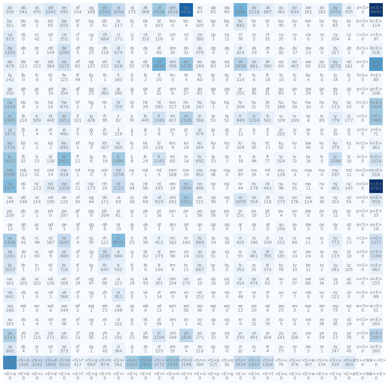
Remove <E> and <S> in favor of a single . token
Will deduct the columns and row having 0 values
stoi = get_stoi(words, '.', '.')
stoi
{ '.': 0, 'a': 1, 'b': 2, 'c': 3, 'd': 4, 'e': 5, 'f': 6, 'g': 7, 'h': 8, 'i': 9, 'j': 10, 'k': 11, 'l': 12, 'm': 13, 'n': 14, 'o': 15, 'p': 16, 'q': 17, 'r': 18, 's': 19, 't': 20, 'u': 21, 'v': 22, 'w': 23, 'x': 24, 'y': 25, 'z': 26 }
itos = dict(map(reversed, stoi.items()))N = create_bigram_matrix(words, '.', '.')N[0, 0]tensor(0, dtype=torch.int32)
plot_matrix(N, itos)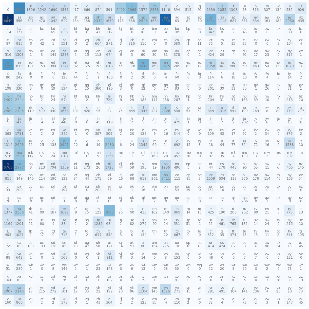
N[0]tensor([ 0, 4410, 1306, 1542, 1690, 1531, 417, 669, 874, 591, 2422, 2963, 1572, 2538, 1146, 394, 515, 92, 1639, 2055, 1308, 78, 376, 307, 134, 535, 929], dtype=torch.int32)
Sampling
Warm up with probability tensor
p = torch.rand(3, generator=g)
ptensor([0.7081, 0.3542, 0.1054])
p.sum()tensor(1.1678)
p = p/p.sum()
ptensor([0.6064, 0.3033, 0.0903])
Drawing 20 samples
p_dist = torch.multinomial(p, num_samples=20, replacement=True, generator=g)
p_disttensor([1, 1, 2, 0, 0, 2, 1, 1, 0, 0, 0, 1, 1, 0, 0, 1, 1, 0, 0, 1])
len(p_dist[p_dist == 0])/len(p_dist)0.45
len(p_dist[p_dist == 1])/len(p_dist)0.45
len(p_dist[p_dist == 2])/len(p_dist)0.1
Drawing 50 samples
p_dist = torch.multinomial(p, num_samples=50, replacement=True, generator=g)
p_disttensor([0, 2, 0, 0, 1, 0, 0, 1, 0, 0, 0, 1, 1, 1, 0, 1, 1, 0, 0, 1, 1, 1, 0, 1, 1, 0, 1, 1, 0, 2, 0, 0, 0, 0, 0, 0, 0, 0, 0, 0, 1, 1, 0, 0, 0, 0, 0, 0, 0, 0])
len(p_dist[p_dist == 0])/len(p_dist)0.64
len(p_dist[p_dist == 1])/len(p_dist)0.32
len(p_dist[p_dist == 2])/len(p_dist)0.04
Drawing a character wrt to probability of occurance
p = N[0].float()
p = p / p.sum()
ptensor([0.0000, 0.1377, 0.0408, 0.0481, 0.0528, 0.0478, 0.0130, 0.0209, 0.0273, 0.0184, 0.0756, 0.0925, 0.0491, 0.0792, 0.0358, 0.0123, 0.0161, 0.0029, 0.0512, 0.0642, 0.0408, 0.0024, 0.0117, 0.0096, 0.0042, 0.0167, 0.0290])
ix = torch.multinomial(p, num_samples=1, replacement=True, generator=g).item()
ix
19
itos[ix]'s'
def generate_names(count, pdist_func, g):
    for i in range(count):
        out = []
        ix = 0
        while True:
            p = pdist_func(ix)
            ix = torch.multinomial(p, num_samples = 1, replacement = True, generator = g).item()
            out.append(itos[ix])
            if ix == 0:
                break
        yield ''.join(out)
p_occurance = lambda ix: N[ix].float()/N[ix].sum()
for name in generate_names(10, p_occurance, g): print(name)blon.
ke.
a.
ry.
l.
balycaweriginnn.
data.
bh.
matt.
jeeve.
Drawing a character wrt to uniform probability
p_uniform = lambda ix: torch.ones(len(N[ix]))/len(N[ix])for name in generate_names(10, p_uniform, g): print(name)wwjieqrrlvhtwogbqtwrmcjpnvrkifgnsgfvp.
kynsszpvqzmmwpogyzdhpfapyhlqdxcvczntn.
.
.
rxnsmepegjipknhbzrrz.
kgkznqqzsdaacfanvedfjga.
ycgfsirvvmcrvssnqjbjuqfzanulmxxkseuktjmbhn.
x.
wsuzuxkneqmel.
qrbcskqqopeqbkuidxrnmyyfvysdxvfwix.
Vectorized normalization of rows and columns
Warm up with normalization
P = N.float()P.shapetorch.Size([27, 27])
P.sum(0, keepdim=True).shapetorch.Size([1, 27])
P.sum(1, keepdim=True).shapetorch.Size([27, 1])
P.sum(0, keepdim=False).shapetorch.Size([27])
P.sum(1, keepdim=False).shapetorch.Size([27])
Broadcasting
Two tensors are “broadcastable” if the following rules hold:
- Each tensor has at least one dimension.
- When iterating over the dimension sizes, starting at the trailing dimension, the dimension sizes must either be equal, one of them is 1, or one of them does not exist.P.shapetorch.Size([27, 27])
P_sum_col = P.sum(1, keepdim=True)
P_sum_col.shapetorch.Size([27, 1])
As you can see above the shapes of the two variables P and P_sum_col are
27 by 27
27 by 1
Broadcasting will repeat the unit dimension of the second variable 27 times along the y axis and it does element wise division
So the P_norm will be
P_norm = P/P_sum_colP_norm.shapetorch.Size([27, 27])
normalized_P = lambda ix: P_norm[ix]for name in generate_names(10, normalized_P, g): print(name)ele.
zelensskan.
a.
ilelena.
arah.
lizanolbraris.
sil.
kyliketo.
asonnngaeyja.
an.
P_sum_col without keepdims
P_sum_col_wo_keepdims = P.sum(1)
P_sum_col_wo_keepdims.shapetorch.Size([27])
And what if we use the variable P_sum_col_wo_keepdims to divide the P, how will the broadcasting rule be applied?
So the shapes of the two variables P and P_sum_col_wo_keepdims are
27 by 27
27
We will arrange the trailing dimension of the P_sum_col_wo_keepdims shape along with the P shape, so it will be
27 by 27
1 by 27
Now broadcasting will copy the unit dimension of the P_sum_col_wo_keepdims along the x-axis 27 times
The result will be
P_norm_wo_keepdims = P/P_sum_col_wo_keepdimstorch.equal(P_norm_wo_keepdims, P_norm)False
So here we are normalizing the columns instead of the rows when broadcasting without keepdims
wrongly_normalized_P = lambda ix: P_norm_wo_keepdims[ix]for name in generate_names(10, wrongly_normalized_P, g): print(name)cishwambitzuruvefaum.
ajorun.
xilinnophajorovebrglmivoublicckyle.
joyquwasooxxentomprtyuquviequzaq.
juxtrcoxluckyjayspttycelllwyddstotyphaxxxwecquxzikoququzynikoposylixxuffruedrkowh.
ju.
ixxxisrielyavrhmidexytzrohauxiexxxxxxzurefffaigtzuzzantallyojoxxxt.
oprghah.
stzldouwinolyselppp.
j.
Loss function
Probability of each pairing
for ch1, ch2 in generate_pairings(words[:3], '.', '.'): print(f'{ch1}{ch2}').e
em
mm
ma
a.
.o
ol
li
iv
vi
ia
a.
.a
av
va
a.
def generate_pairing_probs(words):
    for ch1, ch2 in generate_pairings(words,'.', '.'):
        ix1 = stoi[ch1]
        ix2 = stoi[ch2]
        prob = P_norm[ix1, ix2]
        yield ch1, ch2, prob
for ch1, ch2, prob in generate_pairing_probs(words[:3]): print(f'{ch1}{ch2}: {prob: .4f}').e: 0.0478
em: 0.0377
mm: 0.0253
ma: 0.3899
a.: 0.1960
.o: 0.0123
ol: 0.0780
li: 0.1777
iv: 0.0152
vi: 0.3541
ia: 0.1381
a.: 0.1960
.a: 0.1377
av: 0.0246
va: 0.2495
a.: 0.1960
The individual character probability is
1/270.037037037037037035
which is ~4%.
if the above probability assigned by the bigram model was 1 then the model is sure about what will come will next
Negative Log Likelihood
The product of the above probabilities will determine how the model is performing. As the product of probabilities will be very small, we are taking the log likelihood
Maximum Likelihood \[ ML = a \times b \times c \]
Log Likelihood \[ \log {(a \times b \times c)} = \log {a} + \log {b} + \log {c} \]
def print_prob_logprob(words):
    for ch1, ch2, prob in generate_pairing_probs(words):
        logprob = torch.log(prob)
        print(f'{ch1}{ch2}: {prob: .4f} {logprob: .4f}')
print_prob_logprob(words[:3])
.e: 0.0478 -3.0408
em: 0.0377 -3.2793
mm: 0.0253 -3.6772
ma: 0.3899 -0.9418
a.: 0.1960 -1.6299
.o: 0.0123 -4.3982
ol: 0.0780 -2.5508
li: 0.1777 -1.7278
iv: 0.0152 -4.1867
vi: 0.3541 -1.0383
ia: 0.1381 -1.9796
a.: 0.1960 -1.6299
.a: 0.1377 -1.9829
av: 0.0246 -3.7045
va: 0.2495 -1.3882
a.: 0.1960 -1.6299
Lets sum up all the log probabilities
def log_likelihood(words):
    log_likelihood = 0
    for ch1, ch2, prob in generate_pairing_probs(words):
        log_likelihood += torch.log(prob)
return log_likelihoodlog_likelihood(words[:3])tensor(-38.7856)
The log likelihood will be 0 if all the probabilities will be 1 and will be negative if one of more of the probability will be less than 0. The maximum number the log likelihood will be 1. We want something which can be defined as loss such that higher the amount of inaccurate predictions higher the loss.
So if we take the negative of log likelihood, we will get an increasing number with higher innacuracy.
def negative_log_likelihood(words):
return -log_likelihood(words)negative_log_likelihood(words[:3])tensor(38.7856)
Sometimes we want to normalize the log_likelihood by the count of pairs. Lets do that
def log_likelihood_normalized(words):
    count = 0
    log_likelihood = 0
    for ch1, ch2, prob in generate_pairing_probs(words):
        log_likelihood += torch.log(prob)
        count += 1
return log_likelihood/countlog_likelihood_normalized(words)tensor(-2.4541)
def negative_log_likelihood_normalized(words):
return -log_likelihood_normalized(words)negative_log_likelihood_normalized(words)tensor(2.4541)
So the training loss is 38.7856
Test it on a test data
negative_log_likelihood_normalized(["anubhav"])tensor(3.1186)
negative_log_likelihood_normalized(["anubhavm"])tensor(inf)
It is infinite loss, means that the model will not predict anubhavm
Lets see which pairing is giving infinite prob
print_prob_logprob(["anubhavm"]).a: 0.1377 -1.9829
an: 0.1605 -1.8296
nu: 0.0052 -5.2518
ub: 0.0329 -3.4157
bh: 0.0155 -4.1669
ha: 0.2946 -1.2220
av: 0.0246 -3.7045
vm: 0.0000 -inf
m.: 0.0777 -2.5551
We see that the pairing vm has 0 probability of occurance which leads to infinite loss.
In the following table also m is following v 0 times
plot_matrix(N, itos)
Model Smooting
To add a very small number (fake counts) to the count of pairing so that the likelihood is not 0 and therefore the negative log likelihood is not negative infinity
P = (N + 1).float()The more fake count you add to N, the more uniform model (uniform probabilities) you will have. The less you add the more peak model (model probabilities) you will have
P_sum_col = P.sum(1, keepdim=True)P_norm = P/P_sum_colprint_prob_logprob(["anubhavm"]).a: 0.1376 -1.9835
an: 0.1604 -1.8302
nu: 0.0053 -5.2429
ub: 0.0329 -3.4146
bh: 0.0157 -4.1529
ha: 0.2937 -1.2251
av: 0.0246 -3.7041
vm: 0.0004 -7.8633
m.: 0.0775 -2.5572
negative_log_likelihood_normalized(["anubhavm"])tensor(3.5526)
Neural Network
Create the train set of the bigrams
def generate_training_set(words, start_token='.', end_token='.'):
    xs, ys = [], []
    for ch1, ch2 in generate_pairings(words, start_token, end_token):
        ix1 = stoi[ch1]
        ix2 = stoi[ch2]
        xs.append(ix1)
        ys.append(ix2)
    return xs, ys
xs, ys = generate_training_set(words[:1])xs = torch.tensor(xs); xstensor([ 0, 5, 13, 13, 1])
ys = torch.tensor(ys); ystensor([ 5, 13, 13, 1, 0])
for ch1, ch2 in generate_pairings(words[:1], '.', '.'):
    print(ch1, ch2)
. e
e m
m m
m a
a .
Difference between torch.tensor and torch.Tensor
torch.tensor infers the dtype automatically, while torch.Tensor returns a torch.FloatTensor. I would recommend to stick to torch.tensor, which also has arguments like dtype, if you would like to change the type.
https://stackoverflow.com/a/63116398
xs.dtype, ys.dtype(torch.int64, torch.int64)
xs, ys = generate_training_set(words)xs = torch.Tensor(xs)
ys = torch.Tensor(ys)
xs.dtype, ys.dtype(torch.float32, torch.float32)
One Hot Encoding of the training dataset
import torch.nn.functional as Fxs, ys = generate_training_set(words[:1])
xs = torch.tensor(xs)
ys = torch.tensor(ys)xenc = F.one_hot(xs, num_classes=27)
xenctensor([[1, 0, 0, 0, 0, 0, 0, 0, 0, 0, 0, 0, 0, 0, 0, 0, 0, 0, 0, 0, 0, 0, 0, 0, 0, 0, 0], [0, 0, 0, 0, 0, 1, 0, 0, 0, 0, 0, 0, 0, 0, 0, 0, 0, 0, 0, 0, 0, 0, 0, 0, 0, 0, 0], [0, 0, 0, 0, 0, 0, 0, 0, 0, 0, 0, 0, 0, 1, 0, 0, 0, 0, 0, 0, 0, 0, 0, 0, 0, 0, 0], [0, 0, 0, 0, 0, 0, 0, 0, 0, 0, 0, 0, 0, 1, 0, 0, 0, 0, 0, 0, 0, 0, 0, 0, 0, 0, 0], [0, 1, 0, 0, 0, 0, 0, 0, 0, 0, 0, 0, 0, 0, 0, 0, 0, 0, 0, 0, 0, 0, 0, 0, 0, 0, 0]])
xenc.shapetorch.Size([5, 27])
plt.imshow(xenc)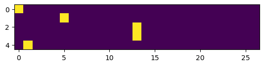
xenc.dtypetorch.int64
When we are sending numbers to NN we dont want the numbers to be int but to be float as it can take various values
xenc = F.one_hot(xs, num_classes=27).float()xenc.dtypetorch.float32
Initialize the weight
W = torch.randn((27, 1))
Wtensor([[-1.0414], [-0.4622], [ 0.4704], [ 0.2034], [ 0.4376], [ 0.8326], [-1.1531], [-0.5384], [-1.5000], [-0.3734], [-0.9722], [ 0.7093], [ 1.6148], [ 0.6154], [ 0.6585], [-1.2100], [-0.4480], [ 2.4709], [ 1.5362], [-0.8239], [-1.8200], [-2.4810], [-1.1249], [ 1.2613], [-0.7899], [-0.3423], [-0.8073]])
W.shapetorch.Size([27, 1])
xenc @ Wtensor([[-1.0414], [ 0.8326], [ 0.6154], [ 0.6154], [-0.4622]])
Initialize random weight of 27 by 27
W = torch.randn((27, 27))
xenc @ Wtensor([[-1.3844e+00, 1.5959e-02, 3.7060e-01, 1.1356e+00, 5.2515e-01, 7.3794e-01, -1.0737e+00, -9.0978e-01, 1.2984e+00, 1.0683e+00, 1.2605e+00, -1.7498e+00, 4.6805e-01, -3.4442e-01, 1.0569e+00, 1.8138e-01, 8.4084e-01, 1.3287e+00, -7.5910e-01, 7.8683e-01, 9.5301e-01, -1.0442e+00, -2.4167e-02, 6.2387e-01, -6.6787e-02, -7.1907e-01, 1.2762e+00], [-9.1542e-01, -8.4699e-02, 8.1029e-01, 5.2382e-01, -1.4164e+00, 9.8146e-01, 2.2023e+00, 5.3777e-01, 2.7927e-01, -5.9158e-03, 1.1951e-01, -1.0505e+00, 2.1483e-01, 4.4787e-01, 1.7172e+00, 1.6195e+00, -1.2666e+00, -4.3973e-01, 7.8754e-02, 2.4022e-01, 5.2765e-01, 3.4238e-01, -1.5155e+00, -3.3794e-02, 1.3747e+00, 1.8808e+00, 3.2315e-01], [ 1.0474e+00, -1.1022e+00, 1.1412e+00, -1.0475e+00, 1.2827e+00, -1.1662e-01, -1.0313e+00, -5.0630e-01, -5.8584e-01, 3.7119e-01, -6.2447e-01, -6.1076e-01, 7.0085e-01, 2.1230e-01, 1.8492e+00, -1.5117e-01, 2.2283e+00, -1.1119e+00, -9.5698e-01, -2.8551e-02, 1.0193e+00, -8.8697e-01, -7.4386e-02, 1.3281e+00, 2.0499e-01, 8.1934e-01, 2.3981e-01], [ 1.0474e+00, -1.1022e+00, 1.1412e+00, -1.0475e+00, 1.2827e+00, -1.1662e-01, -1.0313e+00, -5.0630e-01, -5.8584e-01, 3.7119e-01, -6.2447e-01, -6.1076e-01, 7.0085e-01, 2.1230e-01, 1.8492e+00, -1.5117e-01, 2.2283e+00, -1.1119e+00, -9.5698e-01, -2.8551e-02, 1.0193e+00, -8.8697e-01, -7.4386e-02, 1.3281e+00, 2.0499e-01, 8.1934e-01, 2.3981e-01], [ 1.0060e+00, -1.6259e-02, -1.9179e+00, 1.6954e-02, 1.0129e+00, -8.4792e-01, 1.4553e+00, -8.6143e-01, 3.8685e-01, 7.8658e-01, 1.7895e+00, -3.5575e-01, 4.3668e-01, 4.7369e-01, -1.1651e+00, 5.3522e-02, -2.1702e+00, 1.2975e+00, 1.1129e+00, 8.5445e-01, 2.0814e-01, 2.7412e-01, -2.4321e-04, 1.3574e+00, -4.5190e-01, 1.5984e-01, -1.2650e-01]])
(xenc @ W).shapetorch.Size([5, 27])
(xenc @ W)[3, 13], (xenc[3] * W[:, 13]).sum()(tensor(0.2123), tensor(0.2123))
Exponential
logits = (xenc @ W) # log counts
counts = logits.exp() # counts
countstensor([[0.2505, 1.0161, 1.4486, 3.1130, 1.6907, 2.0916, 0.3418, 0.4026, 3.6636, 2.9104, 3.5272, 0.1738, 1.5969, 0.7086, 2.8773, 1.1989, 2.3183, 3.7761, 0.4681, 2.1964, 2.5935, 0.3520, 0.9761, 1.8661, 0.9354, 0.4872, 3.5830], [0.4003, 0.9188, 2.2486, 1.6885, 0.2426, 2.6683, 9.0457, 1.7122, 1.3222, 0.9941, 1.1269, 0.3498, 1.2396, 1.5650, 5.5687, 5.0507, 0.2818, 0.6442, 1.0819, 1.2715, 1.6949, 1.4083, 0.2197, 0.9668, 3.9539, 6.5587, 1.3815], [2.8502, 0.3321, 3.1304, 0.3508, 3.6062, 0.8899, 0.3565, 0.6027, 0.5566, 1.4495, 0.5355, 0.5429, 2.0155, 1.2365, 6.3550, 0.8597, 9.2838, 0.3289, 0.3841, 0.9719, 2.7713, 0.4119, 0.9283, 3.7739, 1.2275, 2.2690, 1.2710], [2.8502, 0.3321, 3.1304, 0.3508, 3.6062, 0.8899, 0.3565, 0.6027, 0.5566, 1.4495, 0.5355, 0.5429, 2.0155, 1.2365, 6.3550, 0.8597, 9.2838, 0.3289, 0.3841, 0.9719, 2.7713, 0.4119, 0.9283, 3.7739, 1.2275, 2.2690, 1.2710], [2.7347, 0.9839, 0.1469, 1.0171, 2.7535, 0.4283, 4.2858, 0.4226, 1.4723, 2.1959, 5.9862, 0.7006, 1.5476, 1.6059, 0.3119, 1.0550, 0.1142, 3.6601, 3.0433, 2.3501, 1.2314, 1.3154, 0.9998, 3.8861, 0.6364, 1.1733, 0.8812]])
(xenc @ W)[3, 13]tensor(0.2123)
xenc[3]tensor([0., 0., 0., 0., 0., 0., 0., 0., 0., 0., 0., 0., 0., 1., 0., 0., 0., 0., 0., 0., 0., 0., 0., 0., 0., 0., 0.])
W[:, 13]tensor([-0.3444, 0.4737, 0.0557, -0.1620, -0.6734, 0.4479, -0.7111, 1.3282, 0.2026, 0.0208, 0.2722, 0.3473, -0.6560, 0.2123, 1.7973, 1.2086, -1.2879, -0.0824, -1.3538, -0.3161, -0.9458, -1.2972, 0.5641, -0.4949, 1.0295, 0.0753, -0.1173])
(xenc[3] * W[:, 13]).sum() # is equal to (xenc @ W)[3, 13]tensor(0.2123)
logits = xenc @ W # log-counts
counts = logits.exp()
probs = counts / counts.sum(1, keepdims=True)probs.shapetorch.Size([5, 27])
probs[0].sum()tensor(1.)
Summary
xstensor([ 0, 5, 13, 13, 1])
ystensor([ 5, 13, 13, 1, 0])
W = torch.randn((27, 27), generator=g)xenc = F.one_hot(xs, num_classes=27).float()
logits = xenc @ W
counts = logits.exp()
probs = counts/counts.sum(1, keepdims=True)probs.shapetorch.Size([5, 27])
nlls = torch.zeros(5)
for i in range(5):
x = xs[i].item()
y = ys[i].item()
print('-------------------')
print(f'bigram example {i+1}: {itos[x]}{itos[y]} (indexes {x}, {y})')
print('input to the neural network: ', x)
print('output probabilities from the neural net:', probs[i])
print('label (actual next character):', y)
p = probs[i, y]
print('probability assigned by the net to the correct character:', p.item())
logp = torch.log(p)
print('log likelihood:', logp.item())
nll = -logp
print('negative log likelihood:', nll.item())
nlls[i] = nll
print('========')
print('average negtaive log likelihood, i.e. loss = ', nlls.mean().item())-------------------
bigram example 1: .e (indexes 0, 5)
input to the neural network: 0
output probabilities from the neural net: tensor([0.0204, 0.0134, 0.0078, 0.0670, 0.0130, 0.0115, 0.0175, 0.0121, 0.0186, 0.0311, 0.0275, 0.1659, 0.0087, 0.0143, 0.0518, 0.0317, 0.0831, 0.0230, 0.0396, 0.0086, 0.0483, 0.0447, 0.0556, 0.0112, 0.0724, 0.0844, 0.0168])
label (actual next character): 5
probability assigned by the net to the correct character: 0.011521384119987488
log likelihood: -4.463550567626953
negative log likelihood: 4.463550567626953
-------------------
bigram example 2: em (indexes 5, 13)
input to the neural network: 5
output probabilities from the neural net: tensor([0.0081, 0.0690, 0.0499, 0.1331, 0.0985, 0.0740, 0.0093, 0.0052, 0.0234, 0.0321, 0.0267, 0.0309, 0.0093, 0.0228, 0.0269, 0.0085, 0.0049, 0.0363, 0.0139, 0.0326, 0.0531, 0.0262, 0.1151, 0.0097, 0.0136, 0.0420, 0.0248])
label (actual next character): 13
probability assigned by the net to the correct character: 0.0227525494992733
log likelihood: -3.7830779552459717
negative log likelihood: 3.7830779552459717
-------------------
bigram example 3: mm (indexes 13, 13)
input to the neural network: 13
output probabilities from the neural net: tensor([0.0230, 0.0133, 0.0162, 0.0483, 0.0080, 0.0372, 0.0084, 0.0216, 0.0159, 0.0524, 0.0227, 0.0227, 0.0092, 0.0415, 0.1000, 0.0354, 0.0172, 0.0423, 0.0553, 0.0036, 0.0085, 0.0553, 0.0140, 0.0077, 0.0252, 0.2709, 0.0243])
label (actual next character): 13
probability assigned by the net to the correct character: 0.04153481870889664
log likelihood: -3.181223154067993
negative log likelihood: 3.181223154067993
-------------------
bigram example 4: ma (indexes 13, 1)
input to the neural network: 13
output probabilities from the neural net: tensor([0.0230, 0.0133, 0.0162, 0.0483, 0.0080, 0.0372, 0.0084, 0.0216, 0.0159, 0.0524, 0.0227, 0.0227, 0.0092, 0.0415, 0.1000, 0.0354, 0.0172, 0.0423, 0.0553, 0.0036, 0.0085, 0.0553, 0.0140, 0.0077, 0.0252, 0.2709, 0.0243])
label (actual next character): 1
probability assigned by the net to the correct character: 0.013294448144733906
log likelihood: -4.320408821105957
negative log likelihood: 4.320408821105957
-------------------
bigram example 5: a. (indexes 1, 0)
input to the neural network: 1
output probabilities from the neural net: tensor([0.0538, 0.0021, 0.3426, 0.0492, 0.0995, 0.0047, 0.0090, 0.0162, 0.0012, 0.0138, 0.0374, 0.0028, 0.0075, 0.0097, 0.0124, 0.0284, 0.0163, 0.0218, 0.0011, 0.0579, 0.0165, 0.0460, 0.0432, 0.0132, 0.0680, 0.0072, 0.0184])
label (actual next character): 0
probability assigned by the net to the correct character: 0.05381616950035095
log likelihood: -2.9221813678741455
negative log likelihood: 2.9221813678741455
========
average negtaive log likelihood, i.e. loss = 3.734088182449341
Lets have the above one into function and try with different sampling
def train():
xenc = F.one_hot(xs, num_classes=27).float()
logits = xenc @ W
counts = logits.exp()
probs = counts/counts.sum(1, keepdims=True)
nlls = torch.zeros(5)
for i in range(5):
x = xs[i].item()
y = ys[i].item()
p = probs[i, y]
logp = torch.log(p)
nll = -logp
nlls[i] = nll
return nlls.mean().item()W = torch.randn((27, 27))
train()3.5860557556152344
W = torch.randn((27, 27))
train()3.2332470417022705
Forward Pass
xs, ys(tensor([ 0, 5, 13, 13, 1]), tensor([ 5, 13, 13, 1, 0]))
probs[0, 5], probs[1, 13], probs[2, 13], probs[3, 1], probs[4, 0](tensor(0.0115), tensor(0.0228), tensor(0.0415), tensor(0.0133), tensor(0.0538))
torch.arange(5)tensor([0, 1, 2, 3, 4])
probs[torch.arange(5), ys]tensor([0.0115, 0.0228, 0.0415, 0.0133, 0.0538])
probs[torch.arange(5), ys].log()tensor([-4.4636, -3.7831, -3.1812, -4.3204, -2.9222])
probs[torch.arange(5), ys].log().mean()tensor(-3.7341)
loss = - probs[torch.arange(5), ys].log().mean()
losstensor(3.7341)
def train():
    xenc = F.one_hot(xs, num_classes=27).float()
    logits = xenc @ W
    counts = logits.exp()
    probs = counts/counts.sum(1, keepdims=True)
    loss = - probs[torch.arange(5), ys].log().mean()
    return loss
W = torch.randn((27, 27))
train()tensor(3.2426)
Backward Pass
1st pass
W = torch.randn((27, 27), requires_grad=True)W.grad = None # way to set to zero the gradient
loss = train()
loss.backward()losstensor(4.3984, grad_fn=<NegBackward0>)
W.shape, W.grad.shape(torch.Size([27, 27]), torch.Size([27, 27]))
W.grad[:1]tensor([[ 0.0044, 0.0015, 0.0060, 0.0069, 0.0096, -0.1978, 0.0005, 0.0116, 0.0018, 0.0012, 0.0054, 0.0056, 0.0202, 0.0023, 0.0066, 0.0012, 0.0004, 0.0484, 0.0040, 0.0016, 0.0035, 0.0061, 0.0292, 0.0040, 0.0042, 0.0047, 0.0065]])
2nd pass
W.data += -0.1 * W.gradW.grad = None
loss = train()
loss.backward()losstensor(4.3766, grad_fn=<NegBackward0>)
3rd pass
W.data += -0.1 * W.gradW.grad = None
loss = train()
loss.backward()losstensor(4.3549, grad_fn=<NegBackward0>)
Training loop
xs, ys = generate_training_set(words)
xs = torch.tensor(xs)
ys = torch.tensor(ys)
num = xs.nelement()
print("Number of examples ", num)
xenc = F.one_hot(xs, num_classes=27).float()
Number of examples 228146
def train(xenc, ys, epochs, lr = 0.1):
    W = torch.randn((27, 27), requires_grad=True)
    for epoch in range(epochs):
        # forward pass
        logits = xenc @ W
        counts = logits.exp()
        probs = counts/counts.sum(1, keepdims=True)
        loss = - probs[torch.arange(ys.shape[0]), ys].log().mean()
        print('Epoch: ', epoch, 'Loss: ', loss)

        # backward pass
        W.grad = None
        loss.backward()
        W.data += - lr* W.grad
    return W
model = train(xenc, ys, 10, 1)Epoch: 0 Loss: tensor(3.7543, grad_fn=<NegBackward0>)
Epoch: 1 Loss: tensor(3.7461, grad_fn=<NegBackward0>)
Epoch: 2 Loss: tensor(3.7380, grad_fn=<NegBackward0>)
Epoch: 3 Loss: tensor(3.7300, grad_fn=<NegBackward0>)
Epoch: 4 Loss: tensor(3.7221, grad_fn=<NegBackward0>)
Epoch: 5 Loss: tensor(3.7143, grad_fn=<NegBackward0>)
Epoch: 6 Loss: tensor(3.7066, grad_fn=<NegBackward0>)
Epoch: 7 Loss: tensor(3.6990, grad_fn=<NegBackward0>)
Epoch: 8 Loss: tensor(3.6914, grad_fn=<NegBackward0>)
Epoch: 9 Loss: tensor(3.6840, grad_fn=<NegBackward0>)
model = train(xenc, ys, 10, 10)Epoch: 0 Loss: tensor(3.7679, grad_fn=<NegBackward0>)
Epoch: 1 Loss: tensor(3.6911, grad_fn=<NegBackward0>)
Epoch: 2 Loss: tensor(3.6209, grad_fn=<NegBackward0>)
Epoch: 3 Loss: tensor(3.5565, grad_fn=<NegBackward0>)
Epoch: 4 Loss: tensor(3.4974, grad_fn=<NegBackward0>)
Epoch: 5 Loss: tensor(3.4433, grad_fn=<NegBackward0>)
Epoch: 6 Loss: tensor(3.3937, grad_fn=<NegBackward0>)
Epoch: 7 Loss: tensor(3.3482, grad_fn=<NegBackward0>)
Epoch: 8 Loss: tensor(3.3064, grad_fn=<NegBackward0>)
Epoch: 9 Loss: tensor(3.2681, grad_fn=<NegBackward0>)
model = train(xenc, ys, 10, 100)Epoch: 0 Loss: tensor(3.8536, grad_fn=<NegBackward0>)
Epoch: 1 Loss: tensor(3.1448, grad_fn=<NegBackward0>)
Epoch: 2 Loss: tensor(2.9057, grad_fn=<NegBackward0>)
Epoch: 3 Loss: tensor(2.7856, grad_fn=<NegBackward0>)
Epoch: 4 Loss: tensor(2.7163, grad_fn=<NegBackward0>)
Epoch: 5 Loss: tensor(2.6870, grad_fn=<NegBackward0>)
Epoch: 6 Loss: tensor(2.6442, grad_fn=<NegBackward0>)
Epoch: 7 Loss: tensor(2.6310, grad_fn=<NegBackward0>)
Epoch: 8 Loss: tensor(2.6032, grad_fn=<NegBackward0>)
Epoch: 9 Loss: tensor(2.6044, grad_fn=<NegBackward0>)
model = train(xenc, ys, 100, 10)Epoch: 0 Loss: tensor(3.9659, grad_fn=<NegBackward0>)
Epoch: 1 Loss: tensor(3.8651, grad_fn=<NegBackward0>)
Epoch: 2 Loss: tensor(3.7738, grad_fn=<NegBackward0>)
Epoch: 3 Loss: tensor(3.6906, grad_fn=<NegBackward0>)
Epoch: 4 Loss: tensor(3.6145, grad_fn=<NegBackward0>)
Epoch: 5 Loss: tensor(3.5448, grad_fn=<NegBackward0>)
Epoch: 6 Loss: tensor(3.4810, grad_fn=<NegBackward0>)
Epoch: 7 Loss: tensor(3.4227, grad_fn=<NegBackward0>)
Epoch: 8 Loss: tensor(3.3695, grad_fn=<NegBackward0>)
Epoch: 9 Loss: tensor(3.3209, grad_fn=<NegBackward0>)
Epoch: 10 Loss: tensor(3.2766, grad_fn=<NegBackward0>)
Epoch: 11 Loss: tensor(3.2362, grad_fn=<NegBackward0>)
Epoch: 12 Loss: tensor(3.1992, grad_fn=<NegBackward0>)
Epoch: 13 Loss: tensor(3.1654, grad_fn=<NegBackward0>)
Epoch: 14 Loss: tensor(3.1343, grad_fn=<NegBackward0>)
Epoch: 15 Loss: tensor(3.1055, grad_fn=<NegBackward0>)
Epoch: 16 Loss: tensor(3.0788, grad_fn=<NegBackward0>)
Epoch: 17 Loss: tensor(3.0540, grad_fn=<NegBackward0>)
Epoch: 18 Loss: tensor(3.0307, grad_fn=<NegBackward0>)
Epoch: 19 Loss: tensor(3.0089, grad_fn=<NegBackward0>)
Epoch: 20 Loss: tensor(2.9884, grad_fn=<NegBackward0>)
Epoch: 21 Loss: tensor(2.9690, grad_fn=<NegBackward0>)
Epoch: 22 Loss: tensor(2.9507, grad_fn=<NegBackward0>)
Epoch: 23 Loss: tensor(2.9334, grad_fn=<NegBackward0>)
Epoch: 24 Loss: tensor(2.9170, grad_fn=<NegBackward0>)
Epoch: 25 Loss: tensor(2.9015, grad_fn=<NegBackward0>)
Epoch: 26 Loss: tensor(2.8867, grad_fn=<NegBackward0>)
Epoch: 27 Loss: tensor(2.8727, grad_fn=<NegBackward0>)
Epoch: 28 Loss: tensor(2.8594, grad_fn=<NegBackward0>)
Epoch: 29 Loss: tensor(2.8467, grad_fn=<NegBackward0>)
Epoch: 30 Loss: tensor(2.8347, grad_fn=<NegBackward0>)
Epoch: 31 Loss: tensor(2.8232, grad_fn=<NegBackward0>)
Epoch: 32 Loss: tensor(2.8123, grad_fn=<NegBackward0>)
Epoch: 33 Loss: tensor(2.8019, grad_fn=<NegBackward0>)
Epoch: 34 Loss: tensor(2.7920, grad_fn=<NegBackward0>)
Epoch: 35 Loss: tensor(2.7825, grad_fn=<NegBackward0>)
Epoch: 36 Loss: tensor(2.7735, grad_fn=<NegBackward0>)
Epoch: 37 Loss: tensor(2.7649, grad_fn=<NegBackward0>)
Epoch: 38 Loss: tensor(2.7567, grad_fn=<NegBackward0>)
Epoch: 39 Loss: tensor(2.7489, grad_fn=<NegBackward0>)
Epoch: 40 Loss: tensor(2.7414, grad_fn=<NegBackward0>)
Epoch: 41 Loss: tensor(2.7343, grad_fn=<NegBackward0>)
Epoch: 42 Loss: tensor(2.7274, grad_fn=<NegBackward0>)
Epoch: 43 Loss: tensor(2.7209, grad_fn=<NegBackward0>)
Epoch: 44 Loss: tensor(2.7147, grad_fn=<NegBackward0>)
Epoch: 45 Loss: tensor(2.7087, grad_fn=<NegBackward0>)
Epoch: 46 Loss: tensor(2.7030, grad_fn=<NegBackward0>)
Epoch: 47 Loss: tensor(2.6975, grad_fn=<NegBackward0>)
Epoch: 48 Loss: tensor(2.6923, grad_fn=<NegBackward0>)
Epoch: 49 Loss: tensor(2.6873, grad_fn=<NegBackward0>)
Epoch: 50 Loss: tensor(2.6824, grad_fn=<NegBackward0>)
Epoch: 51 Loss: tensor(2.6778, grad_fn=<NegBackward0>)
Epoch: 52 Loss: tensor(2.6734, grad_fn=<NegBackward0>)
Epoch: 53 Loss: tensor(2.6691, grad_fn=<NegBackward0>)
Epoch: 54 Loss: tensor(2.6650, grad_fn=<NegBackward0>)
Epoch: 55 Loss: tensor(2.6611, grad_fn=<NegBackward0>)
Epoch: 56 Loss: tensor(2.6573, grad_fn=<NegBackward0>)
Epoch: 57 Loss: tensor(2.6536, grad_fn=<NegBackward0>)
Epoch: 58 Loss: tensor(2.6501, grad_fn=<NegBackward0>)
Epoch: 59 Loss: tensor(2.6467, grad_fn=<NegBackward0>)
Epoch: 60 Loss: tensor(2.6434, grad_fn=<NegBackward0>)
Epoch: 61 Loss: tensor(2.6403, grad_fn=<NegBackward0>)
Epoch: 62 Loss: tensor(2.6372, grad_fn=<NegBackward0>)
Epoch: 63 Loss: tensor(2.6343, grad_fn=<NegBackward0>)
Epoch: 64 Loss: tensor(2.6314, grad_fn=<NegBackward0>)
Epoch: 65 Loss: tensor(2.6287, grad_fn=<NegBackward0>)
Epoch: 66 Loss: tensor(2.6260, grad_fn=<NegBackward0>)
Epoch: 67 Loss: tensor(2.6235, grad_fn=<NegBackward0>)
Epoch: 68 Loss: tensor(2.6210, grad_fn=<NegBackward0>)
Epoch: 69 Loss: tensor(2.6185, grad_fn=<NegBackward0>)
Epoch: 70 Loss: tensor(2.6162, grad_fn=<NegBackward0>)
Epoch: 71 Loss: tensor(2.6139, grad_fn=<NegBackward0>)
Epoch: 72 Loss: tensor(2.6117, grad_fn=<NegBackward0>)
Epoch: 73 Loss: tensor(2.6096, grad_fn=<NegBackward0>)
Epoch: 74 Loss: tensor(2.6075, grad_fn=<NegBackward0>)
Epoch: 75 Loss: tensor(2.6055, grad_fn=<NegBackward0>)
Epoch: 76 Loss: tensor(2.6035, grad_fn=<NegBackward0>)
Epoch: 77 Loss: tensor(2.6016, grad_fn=<NegBackward0>)
Epoch: 78 Loss: tensor(2.5998, grad_fn=<NegBackward0>)
Epoch: 79 Loss: tensor(2.5980, grad_fn=<NegBackward0>)
Epoch: 80 Loss: tensor(2.5962, grad_fn=<NegBackward0>)
Epoch: 81 Loss: tensor(2.5945, grad_fn=<NegBackward0>)
Epoch: 82 Loss: tensor(2.5928, grad_fn=<NegBackward0>)
Epoch: 83 Loss: tensor(2.5912, grad_fn=<NegBackward0>)
Epoch: 84 Loss: tensor(2.5896, grad_fn=<NegBackward0>)
Epoch: 85 Loss: tensor(2.5881, grad_fn=<NegBackward0>)
Epoch: 86 Loss: tensor(2.5866, grad_fn=<NegBackward0>)
Epoch: 87 Loss: tensor(2.5851, grad_fn=<NegBackward0>)
Epoch: 88 Loss: tensor(2.5837, grad_fn=<NegBackward0>)
Epoch: 89 Loss: tensor(2.5823, grad_fn=<NegBackward0>)
Epoch: 90 Loss: tensor(2.5809, grad_fn=<NegBackward0>)
Epoch: 91 Loss: tensor(2.5796, grad_fn=<NegBackward0>)
Epoch: 92 Loss: tensor(2.5783, grad_fn=<NegBackward0>)
Epoch: 93 Loss: tensor(2.5770, grad_fn=<NegBackward0>)
Epoch: 94 Loss: tensor(2.5757, grad_fn=<NegBackward0>)
Epoch: 95 Loss: tensor(2.5745, grad_fn=<NegBackward0>)
Epoch: 96 Loss: tensor(2.5733, grad_fn=<NegBackward0>)
Epoch: 97 Loss: tensor(2.5721, grad_fn=<NegBackward0>)
Epoch: 98 Loss: tensor(2.5710, grad_fn=<NegBackward0>)
Epoch: 99 Loss: tensor(2.5698, grad_fn=<NegBackward0>)
Prediction
def generate_names(count):
    for i in range(count):
        out = []
        ix = 0
        while True:
            xenc = F.one_hot(torch.tensor([ix]), num_classes=27).float()
            logits = xenc @ model # predict log-counts
            counts = logits.exp()
            p = counts/counts.sum(1, keepdims=True)

            ix = torch.multinomial(p, num_samples=1, replacement=True, generator=g).item()
            out.append(itos[ix])
            if ix == 0:
                break
print(''.join(out))generate_names(5)zriwreisona.
ady.
myonaxrolin.
arravispgoikeen.
arolouliymairekorqgbwyuere.
Evaluate on Valid and Test set
from torch.utils.data import random_splitx_num = xenc.shape[0]xenc.shapetorch.Size([228146, 27])
test_range, valid_range, train_range = random_split(range(x_num),
            [0.1, 0.1, 0.8],
            generator=g)
test_idx = torch.tensor(test_range)
valid_idx = torch.tensor(valid_range)
train_idx = torch.tensor(train_range)len(train_idx), len(valid_idx), len(test_idx)(182516, 22815, 22815)
x_train, y_train = xenc[train_idx], ys[train_idx]
x_valid, y_valid = xenc[valid_idx], ys[valid_idx]
x_test, y_test = xenc[test_idx], ys[test_idx]
x_train.shape, x_valid.shape, x_test.shape(torch.Size([182516, 27]), torch.Size([22815, 27]), torch.Size([22815, 27]))
y_train.shape, y_valid.shape, y_test.shape(torch.Size([182516]), torch.Size([22815]), torch.Size([22815]))
model = train(x_train, y_train, 100, 10)Epoch: 0 Loss: tensor(3.7710, grad_fn=<NegBackward0>)
Epoch: 1 Loss: tensor(3.6776, grad_fn=<NegBackward0>)
Epoch: 2 Loss: tensor(3.5960, grad_fn=<NegBackward0>)
Epoch: 3 Loss: tensor(3.5230, grad_fn=<NegBackward0>)
Epoch: 4 Loss: tensor(3.4572, grad_fn=<NegBackward0>)
Epoch: 5 Loss: tensor(3.3980, grad_fn=<NegBackward0>)
Epoch: 6 Loss: tensor(3.3445, grad_fn=<NegBackward0>)
Epoch: 7 Loss: tensor(3.2964, grad_fn=<NegBackward0>)
Epoch: 8 Loss: tensor(3.2528, grad_fn=<NegBackward0>)
Epoch: 9 Loss: tensor(3.2134, grad_fn=<NegBackward0>)
Epoch: 10 Loss: tensor(3.1774, grad_fn=<NegBackward0>)
Epoch: 11 Loss: tensor(3.1445, grad_fn=<NegBackward0>)
Epoch: 12 Loss: tensor(3.1142, grad_fn=<NegBackward0>)
Epoch: 13 Loss: tensor(3.0862, grad_fn=<NegBackward0>)
Epoch: 14 Loss: tensor(3.0601, grad_fn=<NegBackward0>)
Epoch: 15 Loss: tensor(3.0357, grad_fn=<NegBackward0>)
Epoch: 16 Loss: tensor(3.0128, grad_fn=<NegBackward0>)
Epoch: 17 Loss: tensor(2.9913, grad_fn=<NegBackward0>)
Epoch: 18 Loss: tensor(2.9711, grad_fn=<NegBackward0>)
Epoch: 19 Loss: tensor(2.9520, grad_fn=<NegBackward0>)
Epoch: 20 Loss: tensor(2.9340, grad_fn=<NegBackward0>)
Epoch: 21 Loss: tensor(2.9170, grad_fn=<NegBackward0>)
Epoch: 22 Loss: tensor(2.9009, grad_fn=<NegBackward0>)
Epoch: 23 Loss: tensor(2.8856, grad_fn=<NegBackward0>)
Epoch: 24 Loss: tensor(2.8712, grad_fn=<NegBackward0>)
Epoch: 25 Loss: tensor(2.8575, grad_fn=<NegBackward0>)
Epoch: 26 Loss: tensor(2.8446, grad_fn=<NegBackward0>)
Epoch: 27 Loss: tensor(2.8323, grad_fn=<NegBackward0>)
Epoch: 28 Loss: tensor(2.8206, grad_fn=<NegBackward0>)
Epoch: 29 Loss: tensor(2.8096, grad_fn=<NegBackward0>)
Epoch: 30 Loss: tensor(2.7991, grad_fn=<NegBackward0>)
Epoch: 31 Loss: tensor(2.7892, grad_fn=<NegBackward0>)
Epoch: 32 Loss: tensor(2.7798, grad_fn=<NegBackward0>)
Epoch: 33 Loss: tensor(2.7708, grad_fn=<NegBackward0>)
Epoch: 34 Loss: tensor(2.7623, grad_fn=<NegBackward0>)
Epoch: 35 Loss: tensor(2.7542, grad_fn=<NegBackward0>)
Epoch: 36 Loss: tensor(2.7466, grad_fn=<NegBackward0>)
Epoch: 37 Loss: tensor(2.7392, grad_fn=<NegBackward0>)
Epoch: 38 Loss: tensor(2.7323, grad_fn=<NegBackward0>)
Epoch: 39 Loss: tensor(2.7256, grad_fn=<NegBackward0>)
Epoch: 40 Loss: tensor(2.7193, grad_fn=<NegBackward0>)
Epoch: 41 Loss: tensor(2.7132, grad_fn=<NegBackward0>)
Epoch: 42 Loss: tensor(2.7074, grad_fn=<NegBackward0>)
Epoch: 43 Loss: tensor(2.7019, grad_fn=<NegBackward0>)
Epoch: 44 Loss: tensor(2.6966, grad_fn=<NegBackward0>)
Epoch: 45 Loss: tensor(2.6915, grad_fn=<NegBackward0>)
Epoch: 46 Loss: tensor(2.6866, grad_fn=<NegBackward0>)
Epoch: 47 Loss: tensor(2.6819, grad_fn=<NegBackward0>)
Epoch: 48 Loss: tensor(2.6774, grad_fn=<NegBackward0>)
Epoch: 49 Loss: tensor(2.6731, grad_fn=<NegBackward0>)
Epoch: 50 Loss: tensor(2.6689, grad_fn=<NegBackward0>)
Epoch: 51 Loss: tensor(2.6649, grad_fn=<NegBackward0>)
Epoch: 52 Loss: tensor(2.6610, grad_fn=<NegBackward0>)
Epoch: 53 Loss: tensor(2.6572, grad_fn=<NegBackward0>)
Epoch: 54 Loss: tensor(2.6536, grad_fn=<NegBackward0>)
Epoch: 55 Loss: tensor(2.6501, grad_fn=<NegBackward0>)
Epoch: 56 Loss: tensor(2.6467, grad_fn=<NegBackward0>)
Epoch: 57 Loss: tensor(2.6434, grad_fn=<NegBackward0>)
Epoch: 58 Loss: tensor(2.6402, grad_fn=<NegBackward0>)
Epoch: 59 Loss: tensor(2.6372, grad_fn=<NegBackward0>)
Epoch: 60 Loss: tensor(2.6342, grad_fn=<NegBackward0>)
Epoch: 61 Loss: tensor(2.6313, grad_fn=<NegBackward0>)
Epoch: 62 Loss: tensor(2.6285, grad_fn=<NegBackward0>)
Epoch: 63 Loss: tensor(2.6258, grad_fn=<NegBackward0>)
Epoch: 64 Loss: tensor(2.6231, grad_fn=<NegBackward0>)
Epoch: 65 Loss: tensor(2.6206, grad_fn=<NegBackward0>)
Epoch: 66 Loss: tensor(2.6181, grad_fn=<NegBackward0>)
Epoch: 67 Loss: tensor(2.6156, grad_fn=<NegBackward0>)
Epoch: 68 Loss: tensor(2.6133, grad_fn=<NegBackward0>)
Epoch: 69 Loss: tensor(2.6110, grad_fn=<NegBackward0>)
Epoch: 70 Loss: tensor(2.6087, grad_fn=<NegBackward0>)
Epoch: 71 Loss: tensor(2.6066, grad_fn=<NegBackward0>)
Epoch: 72 Loss: tensor(2.6044, grad_fn=<NegBackward0>)
Epoch: 73 Loss: tensor(2.6024, grad_fn=<NegBackward0>)
Epoch: 74 Loss: tensor(2.6004, grad_fn=<NegBackward0>)
Epoch: 75 Loss: tensor(2.5984, grad_fn=<NegBackward0>)
Epoch: 76 Loss: tensor(2.5965, grad_fn=<NegBackward0>)
Epoch: 77 Loss: tensor(2.5946, grad_fn=<NegBackward0>)
Epoch: 78 Loss: tensor(2.5928, grad_fn=<NegBackward0>)
Epoch: 79 Loss: tensor(2.5910, grad_fn=<NegBackward0>)
Epoch: 80 Loss: tensor(2.5893, grad_fn=<NegBackward0>)
Epoch: 81 Loss: tensor(2.5876, grad_fn=<NegBackward0>)
Epoch: 82 Loss: tensor(2.5860, grad_fn=<NegBackward0>)
Epoch: 83 Loss: tensor(2.5844, grad_fn=<NegBackward0>)
Epoch: 84 Loss: tensor(2.5828, grad_fn=<NegBackward0>)
Epoch: 85 Loss: tensor(2.5812, grad_fn=<NegBackward0>)
Epoch: 86 Loss: tensor(2.5797, grad_fn=<NegBackward0>)
Epoch: 87 Loss: tensor(2.5783, grad_fn=<NegBackward0>)
Epoch: 88 Loss: tensor(2.5768, grad_fn=<NegBackward0>)
Epoch: 89 Loss: tensor(2.5754, grad_fn=<NegBackward0>)
Epoch: 90 Loss: tensor(2.5741, grad_fn=<NegBackward0>)
Epoch: 91 Loss: tensor(2.5727, grad_fn=<NegBackward0>)
Epoch: 92 Loss: tensor(2.5714, grad_fn=<NegBackward0>)
Epoch: 93 Loss: tensor(2.5701, grad_fn=<NegBackward0>)
Epoch: 94 Loss: tensor(2.5689, grad_fn=<NegBackward0>)
Epoch: 95 Loss: tensor(2.5676, grad_fn=<NegBackward0>)
Epoch: 96 Loss: tensor(2.5664, grad_fn=<NegBackward0>)
Epoch: 97 Loss: tensor(2.5652, grad_fn=<NegBackward0>)
Epoch: 98 Loss: tensor(2.5641, grad_fn=<NegBackward0>)
Epoch: 99 Loss: tensor(2.5629, grad_fn=<NegBackward0>)
Evaluate on Valid set
logits_valid = x_valid @ model
counts_valid = logits_valid.exp()
pred_valid = counts_valid/counts_valid.sum(1, keepdims=True)
- pred_valid[torch.arange(x_valid.shape[0]), y_valid].log().mean()tensor(2.5745, grad_fn=<NegBackward0>)
Evaluate on Test set
logits_test = x_test @ model
counts_test = logits_test.exp()
pred_test = counts_test/counts_test.sum(1, keepdims=True)
- pred_test[torch.arange(x_test.shape[0]), y_test].log().mean()tensor(2.5639, grad_fn=<NegBackward0>)
Regularization (Label Smoothing)
Augment the loss function to have a small component (reguliarization loss) to have a smoother distribution of W. To make all W elements 0
To have a uniform probability distribution
(W ** 2).mean()tensor(0.9617, grad_fn=<MeanBackward0>)
def train(xenc, ys, epochs, lr = 0.1, regularization_parameter = 0.01, print_every_epoch=False):
    W = torch.randn((27, 27), requires_grad=True)
    for epoch in range(epochs):
        # forward pass
        logits = xenc @ W
        counts = logits.exp()
        probs = counts/counts.sum(1, keepdims=True)
        loss = - probs[torch.arange(ys.shape[0]), ys].log().mean()
        regularization_loss = regularization_parameter * (W ** 2).mean()
        loss += regularization_loss
        if print_every_epoch:
            print('Epoch: ', epoch, 'Loss: ', loss)

        # backward pass
        W.grad = None
        loss.backward()
        W.data += - lr* W.grad

    print('Loss: ', loss)
    return W
model = train(x_train, y_train, 100, 10, 0.1)Loss: tensor(2.6531, grad_fn=<AddBackward0>)
model = train(x_train, y_train, 100, 10, 1)Loss: tensor(2.8925, grad_fn=<AddBackward0>)
model = train(x_train, y_train, 100, 10, 0.001)Loss: tensor(2.5767, grad_fn=<AddBackward0>)
model = train(x_train, y_train, 100, 10, 0.0001)Loss: tensor(2.5635, grad_fn=<AddBackward0>)